Long Run vs. Short Run
Production function
The quantity of output a firm produces depends on the quantity of inputs
This relationship is known as the firm's production function
Inputs and outputs
Fixed input is an input whose quantity is fixed for a period of time and cannot be varied (ie. Land)
Variable input is an input whose quantity can vary over a short period of time (ie. Labor)
Long run vs. short run
In the long run, there are no fixed inputs. All costs are variable
In the short run, at least one input will be fixed
Marginal Product of Labor (MPL)
Definition
- change in quantity of output produced by one additional unit of labor
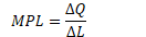
Formula
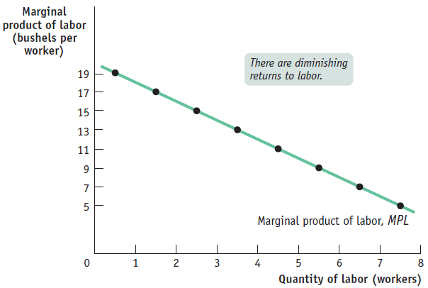
Graph
Downward sloping
Quantity of Labor on the x-axis
MPL of labor on the y-axis
Example 1
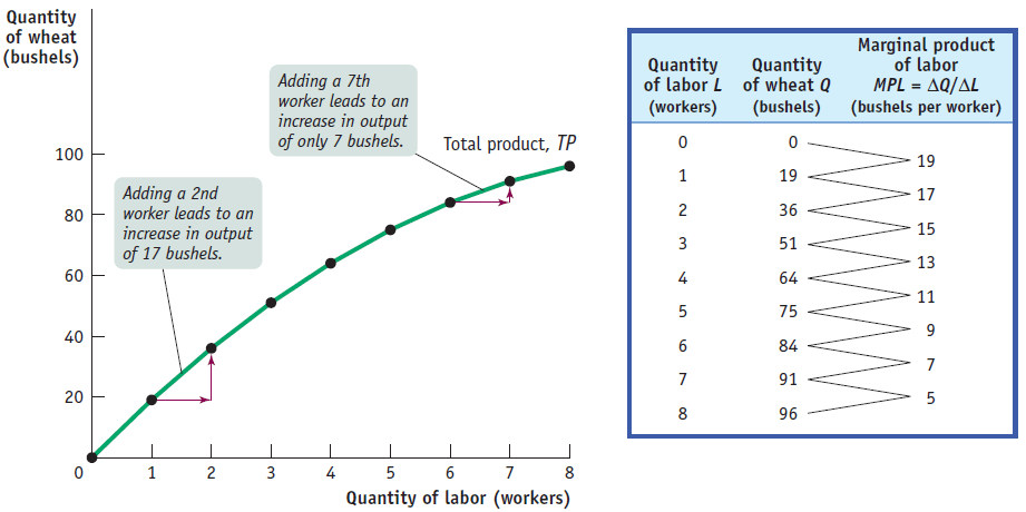
The table shows the production function, the relationship between the quantity of the variable input (labor, measured in number of workers) and the quantity of output (wheat, measured in bushels) for a given quantity of the fixed input.
It also shows the marginal product of labor on George and Martha's farm.
The total product curve shows the production function graphically.
It slopes upward because more wheat is produced as more workers are employed.
It also becomes flatter because the marginal product of labor declines as more and more workers are employed.
The marginal product of labor curve plots each worker's marginal product, the increase in the quantity of output generated by each additional worker.
The change in the quantity of output is measured on the vertical axis and the number of workers employed on the horizontal axis.
The first worker employed generates an increase in output of 19 bushels, the second worker generates an increase of 17 bushels, and so on.
The curve slopes downward due to the diminishing returns to labor
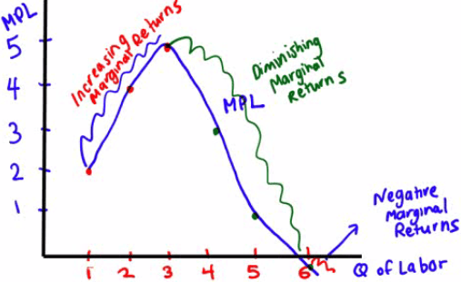
Different Types of Marginal Returns
Increasing marginal returns
- The MPL increases as you hire more workers
Diminishing marginal returns
- The MPL decreases but the total output increases
Negative marginal returns
- The MPL decreases as well as the total output
Graph
Was Thomas Malthus Correct?
In his book, An Essay On the Principle of Population, Thomas Malthus predicted that, based on the principle of diminishing marginal returns, we would have to brace ourselves for a widespread starvation of the masses.
Thomas Carlyle coined the phrase "dismal science" - the term has caught on to describe economics as a gloomy subject
Was Malthus right?
No, he did not account for the increase in TECHNOLOGY!
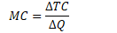
Fixed, Variable and Total Cost
Fixed cost
- cost that does not depend on the quantity of output produced (ie. franchising fee)
Variable cost
- cost that depends on the quantity of output produced (ie. bread, cheese, part-time workers)
Total cost
Sum of fixed and variable cost

Graph
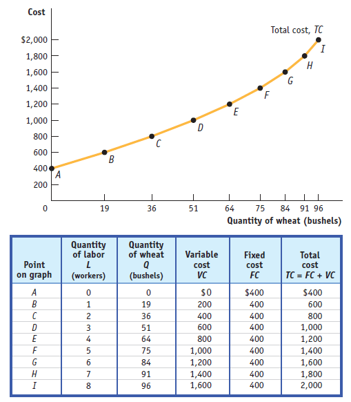
The total cost curve slopes upward because the number of workers employed, and hence total cost, increases as the quantity of output increases.
The curve gets steeper as output increases due to diminishing returns to labor.
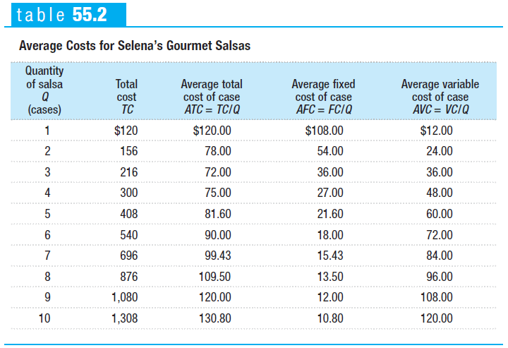
Average Cost
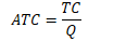
Average total cost
total cost per unit of output
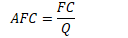
Average fixed cost
fixed cost per unit of output
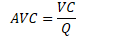
Average variable cost
variable cost per unit of output
Marginal Cost
Meaning
change in total cost generated by one additional unit of output
change in total cost divided by change in quantity of output
Formula
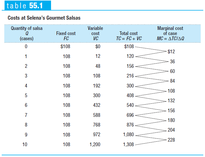
Relationship Between ATC and MC Curves
At the minimum-cost output, average total cost is equal to marginal cost - ALWAYS!
At output less than the minimum-cost output, MC is less than ATC and the ATC is rising
At output greater than the minimum-cost output, MC is greater than ATC and ATC is rising
Ideal Graph
MC: marginal cost
ATC: average total cost
AVC: average variable cost
AFC: average fixed cost
Typical Graph
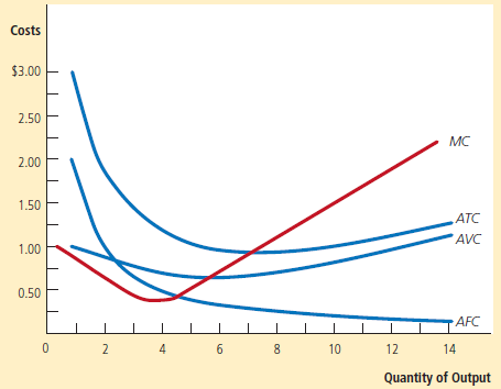
Many firms experience increasing marginal product before diminishing marginal product.
As a result, they have cost curves shaped like those in this figure.
True or False Questions
ATC is always greater than AVC by a constant amount
Answer: False
Reason: The distance between ATC and AVC is AFC
If a firm shuts down in the short run, its profits will equal zero
Answer: False
Reason: Fixed cost is a cost that you will incur even if you shut down
Equations:
Total cost = Fixed cost + Variable cost
Profit = Total revenue - Total cost
Price vs. average variable cost
If P > AVC, stay in business
If P < AVC, then shutdown